Python para ingenieros mecanicos, Ecuacion de transferencia de calor

1. python_examples_mechanical_engineers
2. Heat_transfer.ipynb

Ecuación de transferencia de calor

# Fuente https://firsttimeprogrammer.blogspot.com/

2015/07/the-heat-equation-python-implementation.html 

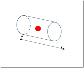
Vamos a simular el transporte de calor a través de una barra ideal .

Supongamos que tiene una varilla cilíndrica cuyos extremos se mantienen a una temperatura fija y se calienta a cierta x durante un cierto intervalo de tiempo. Suponga que la temperatura en cada sección con ancho infinitesimal DX es uniforme para que podamos describir la temperatura en la barra utilizando una función de solo x y t.

Matemáticamente hablando, el problema que ahora nos enfrentamos es el siguiente:

∂ u ∂ t = k ∂ 2 u ∂ x 2 a u ( x , 0 ) = f ( x ) u ( 0 , t ) = u ( l , t ) = 0 0 < t ; 0 ≤ x ≤ l 0 < x < l t > 0 (1) (2) (3)

dónde k

es una constante llamada difusividad térmica o conductividad térmica y es diferente según los diferentes materiales. Al utilizar el método de separación de variables, podemos encontrar la solución que necesitamos y aplicando las condiciones iniciales para encontrar una solución particular f ( x ) = s i n ( x ) y L = P I

Nuestra solución se parece a esto:

u ( x , t ) = e - k t sin ( x )

Ahora solo necesitamos evaluar nuestra función en cada X y T. Recuerde que si u (x, y) es diferenciable, entonces:

F ( x 0 + h , t 0 + l ) = f ( x 0 , t 0 ) + ∂ u ∂ x ( x 0 , t 0 ) h + u - ( t 2 x 0 , t 0 ) l + o h - - √ - l - 2 + - ( ∂ ​ ​

sostiene. Podemos tirar el último término y aproximar nuestra función utilizando la relación anterior, ya que las derivadas parciales de U deben existe y podemos obtenerlas fácilmente. Pensando en ello, el segundo término también es inútil, ya que no nos estamos moviendo a lo largo del eje x, por lo tanto, nos queda lo siguiente:

f ( x 0 + h , t 0 + l ) ≈ f ( x 0 , t 0 ) + ∂ u ∂ t ( x 0 , t 0 ) l

>>import numpy as np
>>from numpy import pi
>>import matplotlib.pyplot as plt
>>import matplotlib.animation as animation

>>fig = plt.figure()
>>fig.set_dpi(100)
>>ax1 = fig.add_subplot(1,1,1)

>>#Diffusion constant
>>k = 2

>>#Scaling factor (for visualisation purposes)
>>scale = 5

>>#Length of the rod (0,L) on the x axis
>>L = pi

>>#Initial contitions u(0,t) = u(L,t) = 0. Temperature at x=0 and x=L is fixed
>>x0 = np.linspace(0,L+1,10000)
>>t0 = 0
>>temp0 = 5  #Temperature of the rod at rest (before heating)

>>#Increment
>>dt = 0.01

>>#Heat function
>>def u(x,t):
>>    return temp0 + scale*np.exp(-k*t)*np.sin(x)

>>#Gradient of u
>>def grad_u(x,t):
                               #du/dx              #du/dt
>>    return scale*np.array([np.exp(-k*t)*np.cos(x),-k*np.exp(-k*t)*np.sin(x)])

>>a = []
>>t = []

>>for i in range(500):
>>    value = u(x0,t0) + grad_u(x0,t0)[1]*dt
>>    t.append(t0)
>>    t0 = t0 + dt
>>    a.append(value)

>>k = 0
>>def animate(i):         #The plot shows the temperature evolving with time
>>    global k            #at each point x in the rod
>>    x = a[k]            #The ends of the rod are kept at temperature temp0
>>    k += 1              #The rod is heated in one spot, then it cools down
>>    ax1.clear()
>>    plt.plot(x0,x,color='red',label='Temperature at each x')
>>    plt.plot(0,0,color='red',label='Elapsed time '+str(round(t[k],2)))
>>    plt.grid(True)
>>    plt.ylim([temp0-2,2.5*scale])
>>    plt.xlim([0,L])
>>    plt.title('Heat equation')
>>    plt.legend()
    
>>anim = animation.FuncAnimation(fig,animate,frames=360,interval=20)
>>plt.show()